3 Combinatorial Logic

3.1 Combinatorial Circuits

Up to now, we looked at simple logic circuits. These are relatively easy to analyze and synthesize (=develop). The main question in this chapter is: how can we set up and optimize logic circuits?

In the following, we have a look at combinatorial circuits. These are generally logic circuits with

• $n$ inputs $X_0$, $X_1$, … $X_{n-1}$
• $m$ outputs $Y_0$, $Y_1$, … $Y_{m-1}$
• no „memory“, that is: a given set of input bits results in a distinct output

They can be described by

• truth table
• boolean formula
• hardware description language

The ladder one is not the focus of this course.

The applications range:

• (simple) half/full adder
• digital comparators (logic circuit to compare 2 values)
• Multiplexer/demultiplexer
• Arithmetic logic units in microcontrollers and processors
• much more

3.1.1 Example

To understand the synthesis of combinatoric logic we will follow a step-by-step example for this chapter.

Imagine you are working for a company called „mechatronics and Robotics“. One customer wants to have an intelligent switch as an input device connected to a microcontroller for controlling an oven. For this project „Therm-o-Safety“ he needs a combinatoric logic:

• The intelligent switch has 4 user selectable positions: $1$, $2$, $3$, $4$
• Additionally there are 2 non-selectable positions in the case of failure.
• The output $Y=1$ will activate temperature monitoring.
• The temperature monitoring has to be active for $3$ and $4$ in case of a major failure. A major failure is for example when the switch position is unclear. In this case, the input of the combinatorial circuit is „ON“.
• There are no other cases of inputs.

These requirements are put into a truth table:

Abbildung 2 shows one implementation of these requirements. The inputs 001 … 011 represent the inputs $1$…$4$. The cases of failure are coded with 110 and 111.
The output $Y$ is activated as requested. For the two combinations 000 and 101 there is no output value defined. Depending on the requirements for a project these shall either better be 0 or 1 or the output of these does not matter. We had this „does not matter“ before: the technical term is „I don't care“, and it is written as a - or a x.

By this, we have done the first step to synthesize the requested logic.

3.1.2 Sum-of-Products

Now, we want to investigate some of the input combinations (= lines in the truth table). At first, we have a look at the input combination 011, where the output has to be $Y=1$.

If this input combination would be the only one for the output of $Y=1$, the following could be stated:
„$Y=1$ (only) when the $X_0$ is $1$ AND $X_1$ is $1$ AND $X_2$ is $0$ “. It can also be re-arranged to:
„$Y=1$ (only) when the $X_0$ is $1$ AND $X_1$ is $1$ AND $X_2$ is not $1$ “.

This statement is similar to $X_0 \cdot X_1 \cdot \overline{X_2}$. The used conjunction results only in $1$ when all inputs are $1$. The negation of $X_2$ takes account of the fact, that $X_2$ has to be $0$.

Abbildung 3 shows the boolean expression for this combination. In Abbildung 4, this boolean expression is converted into a structure with logic gates.

With the same idea in mind, we can have a look at the other combinations resulting in $Y=1$. These are the combinations 100 and 111:

• For 100 The statement would be: „$Y=1$ (only) when the $X_0$ is $0$ AND $X_1$ is $0$ AND $X_2$ is $1$“. Similarly to the combination above this leads to: $\overline{X_0} \cdot \overline{X_1} \cdot {X_2}$.
• For 111, the boolean expression is ${X_0} \cdot {X_1} \cdot {X_2}$.

In Abbildung 5 all minterms for $Y=1$ are shown. The Abbildung 6 depicts all the logic circuits for the three minterms. These lead to the outputs $Y'$, $Y''$, and $Y'''$.

For the final step, we have to combine the single results for the minterms. The output has to be $1$ when at least one of the minterms is $1$. Therefore, the minterms have to be connected disjunctive:

\begin{align*} Y &= & Y' & \quad + & Y'' & \quad + & Y''' \\ Y &= & (X_0 \cdot X_1 \cdot \overline{X_2}) & \quad + & (\overline{X_0} \cdot \overline{X_1} \cdot {X_2}) & \quad + & ({X_0} \cdot {X_1} \cdot {X_2}) \\ \end{align*}

This leads to the logic circuit shown in Abbildung 7. Here, you can input the different combinations by clicking on the bits of the input nibble.

We have seen, that the sum-of-products is one tool to derive a logic circuit based on a truth table. Alternatively, it is also possible to insert an intermediate step, where the logic formula is simplified.

In the following one possible optimization is shown:

3.1.3 Product-of-Sums

In the sub-chapter before we had a look at the combinations which generate an output of $Y=1$ using the AND operator. Now we are investigating the combinations with $Y=0$. Therefore, we need an operator, which results in $0$ for only one distinct combination.

The first combination to look for is 001. If this input combination would be the only one for the output of $Y=0$, the following could be stated:
„$Y=0$ (only) when the $X_0$ is $1$ AND $X_1$ is $0$ AND $X_2$ is $0$ “.
With having the duality in mind (see chapter The Set of Rules) the opposite is also true:
„$Y=1$ when $X_0$ is $0$ OR $X_1$ is $1$ OR $X_2$ is $1$ “

This is the same as: $\overline{X_0} + X_1 + X_2$
The boolean operator we need here is the OR operator.

Similarly, the combinations 010 and 110 can be transformed. Keep in mind, that this time we are looking for a formula with results in $0$ only for the given one distinct combination.

The Abbildung 8 shows all the maxterms for the Therm-o-Safety example.

The formulas of Abbildung 8 can again be transformed into gate circuits (Abbildung 9). Here, only for the inputs 001, 010, 110 one of the outputs $Y'$, $Y''$ or $Y'''$ is $0$.

When these intermediate outputs $Y'$, $Y''$, and $Y'''$ are used as an input for an AND-gate the resulting output will get $0$ when at least one of the intermediate outputs is $0$. This results in another way to synthesize the Therm-o-Safety (see Abbildung 10)

Also, the product-of-sum can be simplified:

\begin{align*} Y &= & (\overline{X_0} + X_1 + X_2) & \quad \cdot & ({X_0} + \overline{X_1} + X_2) & \quad \cdot & (\overline{X_0} + \overline{X_1} + X_2) \\ &= & ... \\ Y &= & (\overline{X_0} + X_1 + X_2) & \quad \cdot & (\overline{X_1} + \overline{X_2}) \\ \end{align*}

This result from $Y$ by the sum-of-products is different compared to the result in a product-of-sums:

• product-of-sums: $Y = (\overline{X_0} \cdot \overline{X_1} \cdot {X_2}) + (X_0 \cdot X_1)$
• sum-of-products: $Y = (\overline{X_0} + X_1 + X_2) \cdot (\overline{X_1} + \overline{X_2})$

In this case, these results cannot be transformed into each other using boolean rules. This is because the don't-care-terms are used in one case as $1$ in the other as $0$.

3.2 Karnaugh Map

3.2.1 Introduction with the two dimensional Map

For a simple introduction, we take one step back and look at a simple example. The formula $Y(X_1, X_0) = X_0 \cdot X_1$ combines two variables. Therefore, it has two dimensions. In Abbildung 11 (a) the truth table of this is shown. The leftmost column shows the decimal interpretation of the binary numeral given by $X_1$, $X_0$ (e.g. $(X_1=1, X_0=0) \rightarrow 10_2=2_{10}$).

The given logic expression can also be interpreted in a coordinate system, with the following conditions:

• There are only two coordinates on each axis possible: 0 and 1.
• There are as many axes as variables given in the logic: For the example, we have two variables $X_0$ and $X_0$. These are spanning a two-dimensional system.
• On the possible positions, the results $Y$ have to be shown.

In the following pictures of this representation, the values are shown:

• green dot, when the result is 1
• red dot, when the result is 0
• grey dot, when the result is don't care

For the given example the coordinate system shows four possible positions: These are the edges of a square (Abbildung 11 (b)).

We will in the future write this as in Abbildung 11 (c). This diagram is also called karnaugh map (often called k-map or KV map). In the shown Karnaugh map the coordinate $X_0$ is shown vertically and $X_1$ horizontally. Similar to the coordinate system the upper left cell is for $X_1=0$ and $X_0=0$. The upper right cell is for $X_1=1$ and $X_0=0$, and the lower right one is for $X_1=1$ and $X_0=1$. In each cell the result $Y(X_1, X_0)$ is shown as a large number - similar to the color code in the coordinate system. The small number is the decimal representation of the number given by $X_1$ and $X_0$. This index is often not explicitly shown in the Karnaugh map, but it simplifies the fill-in of the map and helps for the start.

The Karnaugh map will help us in the following to find simplifications of more complex logic expressions.

3.2.2 The three-dimensional Karnaugh Map

In this subchapter, we will have a look at our example of thermo--safety. For this example, we found two possible gate logic which can produce the required output. We have also seen, that optimizing the terms (i.e. the min- or maxterms) is often possible. However, we do not know how we can find the optimum implementation.

For this, we try to interpret the inputs of our example again as dimensions in a multidimensional space. The three input variables $X_0$, $X_1$, $X_2$ span a 3-dimensional space. The point 000 is the origin of this space. The three combinations 001, 010, 100 are onto the $X_0$-, $X_1$-, and $X_2$-axis, respectively (see Abbildung 12 (a)). The other combinations can be reached by adding these axis values together (see Abbildung 12 (b)+(c)). This is similar to the situation of a two-dimensional or three-dimensional vector. Three inputs result in this representation in the edges of a cube.

In the Abbildung 12 (d) the situation $X_0=1$, $X_1=1$, $X_2=0$ is shown.

There is also an alternative way to look at this representation:

• The formula $Y=1$ (independent from inputs $X_0...X_{n-1}$) lead to all positions are 1
• A single input equal 1 ( $Y:\, X_0=1$, independent from all other inputs, i.e. all others are don't care) leads in the three-dimensional example to the edges of a side surface of the cube.
  In out example $\color{violet}{X_1=1}$ lead to the situation shown in Abbildung 13 (a). When investigating the shown green dots 010, 011, 110, 111 it is visible that the middle value (= the value for $X_1$) is the same.
  Generally: A single input equal 1 (independent from all other inputs) leads to a structure one dimension smaller than the number of inputs (In our example: 3 inputs $\rightarrow$ two-dimensional structure = surface).
• Multiple given inputs equal 1 lead to smaller structures correspondingly. In our example: $\color{blue}{X_0=1}$ and $\color{violet}{X_1=1}$ ($=\color{blue}{X_0}\cdot \color{violet}{X_1}$) result in the two edges on a corner of the cube (Abbildung 13 (b)). For these coordinates (011, 111) the last two values are the same.
• A minterm (=1 as an output) in our example is given by the intersection of all surfaces for the individual dimensions. In our example:$\color{blue}{X_0=1}$ and $\color{violet}{X_1=1}$ and $\color{brown}{X_2=0}$ ($=\color{blue}{X_0}\cdot \color{violet}{X_1}\cdot \color{brown}{\overline{X_2} }$) result in the two edges on a corner of the cube (Abbildung 13 (c))

On the right side of Abbildung 13 also the truth table is shown. There, the combinations for each side surface of the cube are marked with the corresponding color.

With this representation in mind, we can simplify other representations much more simply.
One example for this would be to represent the formula: $Y= X_0 \cdot X_1 \cdot \overline{X_2} + X_2 \cdot X_1 + X_0 \cdot X_1 $. By drawing this into the cube one will see that it represents only a side surface of the cube. It can be simplified into $Y=X_1$.

We can also try to interpret our Therm-o-Safety truth table. The Abbildung 14 shows the corresponding cube. The problem here is, that it is a bit unhandy to reduce a three-dimensional cube onto a flat monitor or paper. It will also get more stressful for higher dimensions.

Therefore, we try to find a better way to sketch the coordinates, before we simplify our Therm-o-Safety. For the three-dimensional Karnaugh map, it is a good idea to „unwrap“ the cube. This can be done as shown in Abbildung 15.

Out of the flattened cube, we can derive the three-dimensional Karnaugh map (see Abbildung 16). Generally, there are different ways to show the Karnaugh map.

1. One way is to show the variable names of the dimensions in the corner. Be aware, that the order of the numbers in the horizontal direction is 0,0, 0,1, 1,1, 1,0 and not in ascending order!
2. In other ways, the columns/rows related to the dimension are marked with lines. In this representation, only the TRUE (=1) position of the coordinate is highlighted.

In Abbildung 16 the dimensions are additionally marked with colors.

In the following chapters mainly the visualization shown in Abbildung 16 (b) is used.

With this representation, we can now try to read out the logic terms for the Therm-o-Safety from its Karnaugh map. Abbildung 17 shows the neighboring combinations:

• In light brown the group (011 + 111) resp. position 3 and position 7 are shown. This can be simplified into $X_0 \cdot X_1$
• In light blue the group (101 + 111) resp. position 5 and position 7 are shown. This can be simplified into $X_0 \cdot X_2$. This group seems not to be needed, since 111 is already in the light brown group.
• In light violet the group (000 + 100) resp. position 0 and position 4 are shown. This can be simplified into $\overline{X_0} \cdot \overline{X_1}$

The first two groups are also neighboring cells in the Karnaugh map. For the last one, we have to keep in mind, that we had to cut the surface of the cube to flatten it. Therefore, these cells are also neighboring. This leads to the conclusion, that the borders of the Karnaugh map are connected to opposite borders!

For our example, the result would be: (light brown the group) + (light violet the group) $= X_0 \cdot X_1 + \overline{X_0} \cdot \overline{X_1}$

We also have to remember, that there are multiple permutations to show exactly the same logic assignment. This can be interpreted as other ways to unwrap the cube. The Abbildung 18 shows the variant from before at (a). In the image (b) the coordinates are mixed ($X_0 \rightarrow X_1$, $X_1 \rightarrow X_2$, $X_2 \rightarrow X_0$). In the image (c) the position of the origin is not in the upper left corner anymore.
Independent of the permutation, the grouped cells are always neighboring each other.

3.2.3 Four-Dimensional Karnaugh Map

For the four-dimensional Karnaugh map, the situation becomes more complicated in the classical coordinate system. The respective object would be a four-dimensional hypercube (see Abbildung 19). This is hard to print in a two-dimensional layout like on a website or a page. Here, a four-dimensional Karnaugh map might be a good representation.

To create a four-dimensional Karnaugh map, we first look at how the two and three-dimensional Karnaugh maps can be derived. The Abbildung 20 (a) shows, that the two-dimensional Karnaugh map can be created from a one-dimensional one by folding the table on the x-axis and adding $10_2$ to all values. The additional line is marked with the new dimension $X_1$.

The three-dimensional one is created by folding the table on the y-axis and adding $100_2$ to all values. The additional line is marked with the new dimension $X_2$ (Abbildung 20 (b) ). Be aware, that the $X_0$ marking now has to be extended - it is also folded to the right.

The four-dimensional one is created by folding the table again on the x-axis and adding $100_2$ to all values. The additional line is marked with the new dimension $X_2$ (Abbildung 20 (c) ).

By this, we can visually derive the four-dimensional Karnaough map.

Again, there are alternative ways to show the Karnaugh map. To get the index of each cell one can easily add up the values of the dimension $X_0 ... X_3$. This is shown in an example in Abbildung 21.

To get used to the four-dimensional Karnaugh map, we expand our Therm-o-Safety: Instead of four user-selectable levels for the oven, version 2.0 will have seven. The temperature monitoring ($Y=1$) has to be active starting with level $4$. Additionally, the Therm-o-Safety 2.0 has three non-selectable positions for the case of failure, where the last one needs active temperature monitoring. Some of the combinations (0000, 1000, 1001, 1010, 1011, 1100) are not needed.

The truth table of the new Therm-o-Safety 2.0 is shown in Abbildung 19

Now we can fill the Karnaugh map:

Disjunctive Form

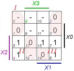
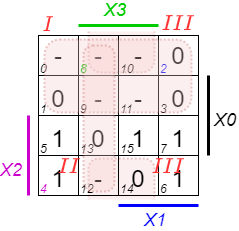
The Karnaugh map can now be used to either get the disjunctive form (= sum-of-products) when looking at the groups of $1$s, or the conjunctive form (= product-of-sums) out of the groups of $0$s. We will first look at the disjunctive form. There are multiple ways to group the minterms. One is shown here:

The group $I$ in Abbildung 24 can be expanded since there are don't care states nearby:

This can be transformed back into a formula. We can derive the boolean terms from the Karnaugh map with the following steps (see Abbildung 26):

1. Investigate every single group individually.
2. For the sum-of-products, each group has to be the product (AND-combination) of the inputs/coordinates.
3. Then the formula can be derived as the sum-of-products…

The given groups are created as a product as follows:

• group $I$: all of this minterms are in the columns of $\color{green}{X_3}$. They are also all in the columns of $\color{blue}{X_1}$ and in the rows of $X_0$. This leads to $X_0 \cdot \color{green}{X_3} \cdot \color{blue}{X_1}$
• group $II$: all of this minterms are in the columns of $\color{green}{\overline{X_3}}$. They are also all in the rows of $\color{magenta}{X_2}$. This leads to $\color{green}{\overline{X_3}} \cdot \color{magenta}{X_2}$

Out of these groups, we can get the full formula by disjunctive combination: \begin{align*} Y &= X_0 \cdot \color{green}{X_3} \cdot \color{blue}{X_1} + \color{green}{\overline{X_3}} \cdot \color{magenta}{X_2} \end{align*}

Conjunctive Form

Similarly, we look at the conjunctive form. Here we have to find groups of $0$s. One way of grouping the maxterms is shown here:

The optimization would be:

Also here, we can derive the boolean terms from the Karnaugh map with the following steps (see Abbildung 29):

1. Investigate every single group individually.
2. For the product-of-sum, each group has to be the sum (OR-combination) of the inputs/coordinates.
   Be aware, that for the OR-combination we get the groups of $0$s as the „rest“ of not-marked cells!
3. In the end, the formula can again be derived, now as the product-of-sums.

\begin{align*} Y &= ( \color{magenta}{X_2}) \cdot( \color{green}{\overline{X_3}} + \color{blue}{X_1}) \cdot( \color{green}{\overline{X_3}} + {X_0}) \end{align*}

Beyond the maxterms this formula can be optimized to

\begin{align*} Y &= \color{magenta}{X_2} \cdot( \color{green}{\overline{X_3}} + (\color{blue}{X_1} \cdot {X_0}) ) \end{align*}

When comparing the disjunctive solution ($X_3 \cdot X_1 \cdot X_0 + \cdot \overline{X_3} \cdot X_2 $) with the conjunctive one ($X_2 \cdot X_1 \cdot X_0 + \cdot \overline{X_3} \cdot X_2 $) we see, that these are definitely different. The given truth table had don't care states. This can be taken as $0$s or $1$s - and therefore combined in groups of $0$s or groups of $1$s.

3.2.4 Rules for the Karnaugh map

We saw, that with the Karnaugh map, we can analyze logic combinations much better. But to use this tool right we have first to look at some definitions.

Allowed Groups

As we have seen, the groups in the Karnaugh map are created by the combination of the inputs. By this, only distinct groups are allowed. These can only have $2^{n-1}$ cells for $n$ inputs (= dimensions).

For a four-dimensional Karnaugh map only the following groups are possible:

• groups of 1: Derived from 4 inputs, e.g. $X_3 \cdot \overline{X_2} \cdot \overline{X_1} \cdot \overline{X_0}$
• groups of 2: Derived from 3 inputs, e.g. $ \overline{X_3} \cdot {X_1} \cdot \overline{X_0}$
• groups of 4: Derived from 2 inputs, e.g. ${X_2} \cdot {X_0}$
• groups of 8: Derived from 1 input , e.g. $\overline{X_1} $

Keep in mind, that not all groups of 2, 4, or 8 cells are allowed. In Abbildung 31 some not allowed groups are shown

Necessary and Important Groups

The sub-chapter before the creation of the groups was done rather intuitively. This shall be explained more structured here. This needs some more definitions.

Abbildung 32 depicts the different implicants in one example.

To get all the necessary implicants the following has to be considered:

• All core prime implicant are needed. They contain terms, which are not covered anywhere else.
• No redundant prime implicant is needed. They are covered by core prime implicants
• Selective prime implicant need to be investigated. Some of them are necessary, depending on the solution (see Abbildung 33)

higher dimensional Karnaugh Maps

For higher dimensional Karnaugh maps the implicants look more am more unintuitive (see Abbildung 34). The Karnaugh map is in our course used to understand the different types of implicants (there will be only three and four-dimensional maps in the exam).

When solving higher dimensional boolean problems the Quine–McCluskey algorithm or a heuristic approach, like the ESPRESSO algorithm can be used. Languages like the Hardware Description Language (HDL) often come with implemented optimizers in the development environment.

Exercises

Exercise 3.1.1 CNF, DNF, Optimization

The following truth table is given.

Abb. 35: Exercise 3.1.1 CNF, DNF, Optimization

1. Write down the DNF for the function table.
Result

For the DNF, one has to only use the following lines to get the minterms:

2. Minimize the DNF step by step, starting with the used boolean rules
Solution steps

\begin{align*} Y &= \overline{X2}\cdot \overline{X1} \cdot X0 + \color{blue}{{X2}\cdot \overline{X1} \cdot X0} + {X2}\cdot {X1} \cdot X0 && | \color{blue}{\text{ Idempotence: Double the second term}} \\ &= \overline{X2}\cdot \overline{X1} \cdot X0 + {X2}\cdot \overline{X1} \cdot X0 + {X2}\cdot \overline{X1} \cdot X0 + {X2}\cdot {X1} \cdot X0 \quad && \\ &= \overline{X2}\cdot \color{blue}{\overline{X1} \cdot X0} + {X2}\cdot \color{blue}{\overline{X1} \cdot X0} + {X2}\cdot \color{violet}{\overline{X1} \cdot X0} + {X2}\cdot \color{violet}{{X1} \cdot X0} \quad && | \color{blue}{\text{Distributive Law }} \color{violet}{\text{(twice)}} \\ &= (\overline{X2}+ X2) \cdot \overline{X1} \cdot X0 + (\overline{X1}+ X1) \cdot {X2} \cdot X0 && \\ &= \color{blue}{(\overline{X2}+ X2)} \cdot \overline{X1} \cdot X0 + \color{violet}{(\overline{X1}+ X1)} \cdot {X2} \cdot X0 && | \color{blue}{\text{ Complementary Element + Neutral Element }} \color{violet}{\text{(twice)}}\\ &= \overline{X1} \cdot X0 + {X2} \cdot X0 && | \color{blue}{\text{ Distributive Law}} \\ &= (\overline{X1} + {X2}) \cdot X0 && \\ \end{align*}

Result

The final result is \begin{align*} Y = (\overline{X1} + {X2}) \cdot X0 \end{align*}

3. Write down the CNF for the function table
Result

For the CNF, one has to only use the following lines to get the maxterms:

4. Minimize the CNF step by step, starting with the used boolean rules
Solution steps

\begin{align*} Y &= (X2 + X1 + X0)_{\color{blue}{I}} \cdot \color{blue}{(X2 + \overline{X1} + X0)}_{\color{blue}{II}} &&\cdot (X2 + \overline{X1} + \overline{X0})_{\color{blue}{III}} \cdot (\overline{X2} + X1 + X0)_{\color{blue}{IV}} &&\cdot (\overline{X2} + \overline{X1} + X0)_{\color{blue}{V}} && | \color{blue}{\text{ Idempotence: Double the second term (II)}} \\ &= (X2 + X1 + X0)_{\color{blue}{I}} \cdot (X2 + \overline{X1} + X0)_{\color{blue}{II}} &&\cdot (X2 + \overline{X1} + \overline{X0})_{\color{blue}{III}} \cdot (\overline{X2} + X1 + X0)_{\color{blue}{IV}} &&\cdot (\overline{X2} + \overline{X1} + X0)_{\color{blue}{V}} \cdot (X2 + \overline{X1} + X0)_{\color{blue}{II}} &&| \text{Commutative Law: rearrange the terms} \\ &= (X2 + X1 + X0)_{\color{blue}{I}} \cdot (\overline{X2} + X1 + X0)_{\color{blue}{IV}} &&\cdot (X2 + \overline{X1} + X0)_{\color{blue}{II}} \cdot (X2 + \overline{X1} + \overline{X0})_{\color{blue}{III}} &&\cdot (\overline{X2} + \overline{X1} + X0)_{\color{blue}{V}} \cdot (X2 + \overline{X1} + X0)_{\color{blue}{II}}\\ &= (X2 + \color{blue}{X1 + X0})_{\hphantom{I}} \cdot (\overline{X2} + \color{blue}{X1 + X0})_{\hphantom{IV}} &&\cdot (\color{violet}{X2 + \overline{X1}} + X0)_{\hphantom{II}} \cdot (\color{violet}{X2 + \overline{X1}} + \overline{X0})_{\hphantom{III}} &&\cdot (\overline{X2} + \color{green}{\overline{X1} + X0})_{\hphantom{V}} \cdot (X2 + \color{green}{\overline{X1} + X0})_{\hphantom{II}} &&| \color{blue}{\text{Distributive Law (}} \color{violet}{\text{three }} \color{green}{\text{times}} \color{black}{\text{)}} \\ &= (X1 + X0) \cdot (X2 + \overline{X2}) &&\cdot (X2 + \overline{X1}) \cdot (X0 + \overline{X0}) &&\cdot (\overline{X2} + X2) \cdot (\overline{X1} + X0) \\ &= (X1 + X0) \cdot \color{blue}{(X2 + \overline{X2})} &&\cdot (X2 + \overline{X1}) \cdot \color{violet}{(X0 + \overline{X0})} &&\cdot \color{green}{(\overline{X2} + X2)} \cdot (\overline{X1} + X0) &&| \color{blue}{\text{ Complementary Element + Neutral Element (}} \color{violet}{\text{three }} \color{green}{\text{times}} \color{black}{\text{)}} \\ &= (X1 + X0) \cdot (X2 + \overline{X1}) \cdot (\overline{X1} + X0) \\ &= (\color{blue}{X1} + X0) \cdot (X2 + \overline{X1}) \cdot (\color{blue}{\overline{X1}} + X0) && && &&| \color{blue}{\text{Distributive Law}}\\ &= (X1 + \overline{X1}) \cdot X0 \cdot (X2 + \overline{X1}) \\ &= \color{blue}{(X1 + \overline{X1})} \cdot X0 \cdot (X2 + \overline{X1}) && && &&| \color{blue}{\text{Complementary Element + Neutral Element}}\\ &= X0 \cdot (X2 + \overline{X1}) \\ \end{align*}

Result

The final result is \begin{align*} Y = (\overline{X1} + {X2}) \cdot X0 \end{align*}

5. Show, that the un-minimized DNF can be converted into the un-minimized CNF (duality principle)
Solution Steps

The distributive law ($a\cdot(b+c)=a\cdot b + a \cdot c$) can be generalized - similar to the conventional algebra: \begin{align*} (a+b)\cdot(c+d) = a\cdot c + a \cdot d + b\cdot c + b\cdot d \end{align*}

This also works for the dual situation: \begin{align*} (a\cdot b)+(c \cdot d) = (a + c) \cdot (a + d) \cdot (b + c) \cdot (b + d) \end{align*}

This can be applied to the DNF: \begin{align*} Y &= \overline{X2}\cdot \overline{X1} \cdot X0 + \color{blue}{{X2}\cdot \overline{X1} \cdot X0} + {X2}\cdot {X1} \cdot X0 \end{align*}

6. Create a Karnaugh map and mark the smallest number of the largest prime implicants. Derive the minimized DNF and CNF from the map.
Result